Peak Detection Using LabVIEW and Measurement Studio

Peak detection is one of the most important time-domain functions performed in signal monitoring. Peak detection is the process of finding the locations and amplitudes of local maxima and minima in a signal that satisfies certain properties. These properties can be simple or complex. For example, requiring that a peak exceeds a certain threshold value is a simple property. However, requiring that a peak’s shape resembles that of a prototype peak is a complex property.

Peak detection is important in many applications, such as chemistry, biology, and music. Scientists and engineers who use analysis techniques such as spectroscopy, chromatography, and tone detection often use peak detection methods specific to those analysis techniques. However, this document describes a general method that applies to a variety of signal types. This is the method used in LabVIEW and Measurement Studio for peak detection functions.

In some applications, you do not need to know the exact peak amplitudes and locations, rather you need to know the number or general locations of peaks. In this case, use a threshold peak detection function, such as the Threshold Peak Detector VI in LabVIEW.

Figure 1 shows the Threshold Peak Detector VI and the VI's inputs and outputs. The VI scans the input sequence X, searches for valid peaks, and keeps track of the indices of the beginnings of the peaks and the total number of peaks found. A peak is considered valid if it has the following characteristics:

• The elements of X begin below threshold, exceed threshold at some index, and then return to a value below threshold
• The number of successive elements that exceed threshold is greater than or equal to width.

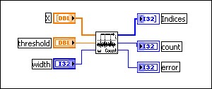
Figure 1. Threshold Peak Detector VI

This VI does not identify the locations or the amplitudes of peaks with great accuracy, but the VI does give an idea of where and how often a signal crosses above a certain threshold value.

The following graph shows a multitone signal after being scanned by the Threshold Peak Detector VI. The input parameters are threshold = 1.00 and width = 10. The VI identifies two peaks, located at approximately 15 and 47. The locations at which they cross the threshold are marked by black dots in Figure 2. However, the VI fails to identify the third potential peak, which crosses the threshold at approximately 132, because it is not at least 10 points wide.

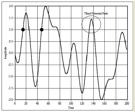
Figure 2. Threshold peak detection performed on a multitone signal, with the parameters set to threshold = 1.00 and width = 10

This VI has some limited but important applications. It is important to understand the distinction between this VI and that of the Peak Detector VI, which is described below.

Some applications require more robust and accurate peak detection algorithms. The rest of this document focuses on uses of advanced peak detection functions, tips to keep in mind and pitfalls to avoid while using them, and methods for ensuring that your peak detection measurements are accurate and useful.

The following sections focus mainly on peaks. However, except where noted, the same information can be used for finding valleys or local minima.

Figure 3 shows the Peak Detector VI and the VI's inputs and outputs. Figure 4 shows the equivalent function prototype in the Advanced Analysis library of LabWindows/CVI.

Figure 3. Peak Detector VI

Figure 4. PeakDetector function prototype for LabWindows/CVI

Notice that it takes handles to the locations, amplitudes, and second derivatives arrays. For descriptions of each of the inputs and outputs for the Peak Detector VI or the PeakDetector function, refer to the LabVIEW or Measurement Studio online help.

LabVIEW also contains a Waveform Peak Detection VI as shown in Figure 5.

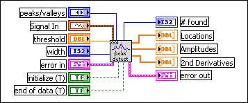
Figure 5. Waveform Peak Detection VI

The Waveform Peak Detection VI operates like the array-based Peak Detector VI. The difference is that this VI's input is a waveform data type, and the VI has error cluster input and output terminals. Locations displays the output array of the peaks or valleys, which is still in terms of the indices of the input waveform. For example, if one element of Locations is 100, that means that there is a peak or valley located at index 100 in the data array of the input waveform. Figure 6 shows you a method for determining the times at which peaks or valleys occur. The following equation locates the peaks and valleys:

Time Locations[i] = t0 + dt* Locations[i]


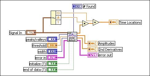
Figure 6. Using the Waveform Peak Detection VI to determine the times at which peaks or valleys occur

The peak detector functions used in LabVIEW and Measurement Studio have some important features that you need to understand before using them. If you use these features correctly, you can actually increase the accuracy and usefulness of peak detection measurements.

1. The function can process many blocks of data that are part of the same signal. By correctly using the initialize (T) and end of data (T) inputs, you can use the peak detection function to analyze a signal that has been broken up into several data blocks. You can also acquire a continuous signal and process pieces of the signal as they become available. The VI finds the peak locations in each block, relative to the previously analyzed blocks. For example, to process a signal acquired in five consecutive blocks, you can use the following pseudocode algorithm:

for i = 1 to 5

[Acquire data]

if (i == 1)
Initialize = True
else
Initialize = False;

if (i == 5)
EndOfData = True
else
EndOfData = False;

Set polarity (peaks or valleys), width, threshold

Call PeakDectector function

Copy the output values to different variables so they will not be overwritten during the next iteration.

next i

The same algorithm in LabVIEW might look like the VI in Figure 7.

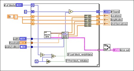
Figure 7. Using the Waveform Peak Detection VI to process a signal that is broken into several blocks

This algorithm uses shift registers and the Build Array function so that the final outputs are still 1D arrays. In this diagram, the Acquire Data VI is generic and used only for illustration.

This multiple-block feature allows you to acquire and analyze data as it becomes available. The data blocks do not have to be all the same size, nor do they have to be acquired at regular time intervals.

2. The function retains internal states and history information from one call to the next. The VI internally allocates the structures that contain this information on the first block of data, and destroys it on the last block of data. Therefore, you must correctly use the initialize (T) and end of data (T) parameters on the first and last data blocks, as illustrated in the pseudocode above.

The function retains history information; it uses a history buffer to retain a certain number of data points from the previous data block. This feature allows the function to correctly locate peaks and valleys that are close to the boundary between blocks. However, you must set end of data (T) and initialize (T) when you have finish analyzing one signal and are starting a new one. Otherwise the function will view the two blocks as part of the same continuous signal and will incorrectly locate peaks or valleys near the end of the last block of the previous signal, or near the beginning of the first block of the new signal.

3. The peak location function gives peak locations at fractional indices. It uses the quadratic fit algorithm and returns the peak locations as floating point numbers, not as integer index values. Therefore, the peak locations and amplitudes usually do not correspond to actual data points in the sampled input signal.

This feature is an advantage of the algorithm because it effectively interpolates between the data points while finding peaks and valleys. The function can therefore measure peaks that have a greater amplitude than any data points near the peak. This interpolation provides a good indication of the true value of the peak in the original analog signal.

4. The function allows implicit noise reduction while finding the peaks. Using the width parameter in some cases can effectively reduce the noise in the input signal when finding the peaks. The minimum value is three; using this value results in no noise reduction. Using a width value larger than three implicitly smooths the data. This feature is useful in some applications. However, you must ensure that you use large width only on noisy data. You must also check to see if the peak locations and amplitude results are reasonable.

5. The function performs a quadratic curve fitting to find the peaks and valleys. The core of the peak-finding algorithm consists of fitting a parabola to successive groups of points, equal in number to width. The function uses the coefficients from the fit to determine whether a peak or valley is present.

If width = 3, then the fit is exact, meaning the parabola will actually pass through each of the three points. If width is greater than three, then a least-squares fit is performed. This process will smooth high-frequency noise if the width is sufficiently large.

For each set of points, the algorithm performs the least-squares quadratic fit, and then performs a series of tests on the coefficients to see whether they meet the criteria for a peak. The function checks whether each parabola is at a local maximum, determines the sign of the quadratic coefficient, which indicates the parabola’s concavity, and finally checks that the peak is above the designated threshold.

To use the peak detection function correctly, you need to have some prior knowledge about your signal. The following are some important issues to consider when specifying the input parameters:

• Is the data a time-domain or a frequency-domain signal?
  If the data is a frequency domain signal and contains one or more well-defined frequency components, use the Power & Frequency Estimate VI in LabVIEW or the PowerFrequencyEstimate function in Measurement Studio. These functions allow you to get more accurate information about the exact frequencies of the peaks and their corresponding energies. LabVIEW 6.0 also includes the Extract Single Tone Information VI, which uses a curve-fitting method to precisely identify the amplitude and frequency of the largest frequency component of a signal.

• Are all the peaks that you are looking for at roughly the same amplitude?
  If so, then set one threshold value for analyzing all the data. However, if you expect to have peaks at many different amplitudes, break up the data and use a different threshold value for separate data blocks.

• Is your data periodic?
  If so, then searching for more than a few periods of the data for peaks is an inefficient use of processing time. Often there is some noise or other distortion present in the data. In this case, average many periods of the original time signal to get one or a few averaged periods, then pass these to the peak detection function.

• Is the data adequately sampled?
  Inadequate sampling of data can result in inaccurate values for the locations and amplitudes of peaks, and the non-detection of valid peaks. Despite the fact that peak detection is essentially a time-domain operation, the sampled signal must still satisfy the Nyquist sampling theorem—the sampling rate must be at least twice the largest frequency component in the signal. However, useful digital representation of a signal typically requires a sampling rate between five and ten times the largest frequency component. The front end of the data acquisition system should contain an analog anti-aliasing filter that removes or strongly attenuates components above Nyquist sampling rate, or half the sampling rate.
  
• Is your data noisy?
  This is a common problem that you must deal with very carefully in peak detection. Clearly, high-frequency noise results in the detection of a large number of peaks, but typically only a few of these will actually be of interest. In these cases, increase the width parameter to implicitly smooth the data for finding the peaks. Notice that since this process tends to remove high-frequency spikes from the data, increasing width tends to decrease the amplitudes of peaks and increase the amplitudes of valleys. You can also use explicit smoothing or interpolation techniques to effectively reduce noise in your data.

Smoothing can cause problems with the measurements if used incorrectly. You need to conduct some initial testing to determine the optimum width. This means you need to determine the number of data points that will remove a sufficient amount of noise without removing significant features of the original signal. However, since you cannot explicitly see the smoothed data, it is difficult to determine the optimum width through visual verification.

In most cases, it is preferable to smooth or process the data before applying the peak detection function. In that case, use a width of three, which tells the peak detection function to process exactly the signal you passed to it, without any smoothing. This method gives you more control over the smoothing and processing of the original signal. The peak detection function then processes only the signal that you pass to it.

Figures 8a, b, and c illustrate this situation. Figure 8a shows a noisy signal and the peaks detected after running the peak detection function using width = 3. Many spurious peaks are detected, and true, de-noised peaks are difficult to locate.

Figure 8b shows the same signal analyzed by the peak detection function using width = 29, a relatively large value. The function detects only three peaks in this case. These peaks may be correct, but it is difficult to determine whether this peak information is really useful.

Figure 8c shows the signal, smoothed by using the same method as the peak detection algorithm, and then passed to the peak detection function. Now the peaks are clear; the results are reasonable and verifiable.

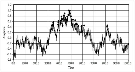
Figure 8a. A noisy waveform after being passed through the peak detection function using width = 3

The black dots mark the detected peaks; most of the marked peaks are not really of interest, but are due to the noise.

The three large black dots are the peak locations returned by the function. It is difficult to tell whether the dots represent accurate amplitudes or locations.

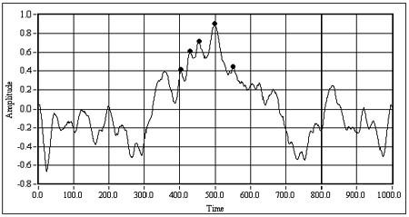
Figure 8c. The same signal as in Figure 8a, using width = 3 , after being smoothed and then analyzed with the peak detection function

The locations of the peaks are clear and the points selected by the algorithm are reasonable.

Since the goal is to obtain accurate locations of peaks and valleys, make sure that any preprocessing of the signal does not shift the signal in time. Such a shift offsets all of the peak location numbers relative to their true locations in the original signal.

Another way to get accurate results from the peak detection functions is interpolation. Interpolation resamples the signal at a higher sampling rate and returns better results.

There are several common methods of interpolating discrete-time signals. A simple method is linear interpolation. If you have an interpolating factor of q, then q-1 points are inserted between each original data point. With linear interpolation, the added points lie on the line through the original data points on either side. While these results are not an accurate representation of the original analog signal, they can help the peak detection algorithm to detect all of the valid peaks.

Another method of interpolation is to interleave q-1 zeros between each of the original data points, then execute a lowpass filter. The theory behind this method is beyond the scope of this document; however, many texts on discrete-time signal processing contain an explanation of this method. For more information on this method, refer to the References section at the end of this document.

A certain trade-off comes with interpolation. Interpolating the digitized signal tends to place the found peaks closer to actual points in the interpolated signal. However, depending on the nature of the analog signal, these may or may not be closer to the real peaks than those detected using the uninterpolated digital signal. So the trade-off is between finding all valid peaks and getting more accurate data for the peak locations and amplitudes.

You now know how to use the peak detection functions in LabVIEW and Measurement Studio to find the locations and amplitudes of peaks and valleys in your signals. The powerful features of these functions lend themselves to convenient and accurate signal analysis. However, as described above, it is important to understand the significance of the input parameters when using the functions. Furthermore, to use these functions effectively, you need to have an understanding of the nature of the input signal before using the peak detector functions.

The resources linked below contain more information about the theory behind methods of digital signal processing, specifically digital filtering, and interpolation. For valuable information about frequency-domain analysis, digital filtering, and using LabVIEW and Measurement Studio to apply the ideas presented in this document, refer to the resources linked below.

You can order the following books through National Instruments Books and Publications linked below:

• Chugani, Mahesh L., Samant, Abhay R., and Cerna, Michael. LabVIEW Signal Processing, Prentice Hall, 1998.
• Haykin, Simon and Van Veen, Barry, Signals and Systems. John Wiley & Sons, Inc., 1998.
• Oppenheim, Alan V. and Schafer, Ronald W. Discrete Time Signal Processing, Prentice Hall, 1999.