Four Practical Applications of Joint Time-Frequency Analysis

Inverse synthetic aperture radar (ISAR) is an imaging radar that uses the target’s pitch, roll and yaw motions to generate an image in the range-Doppler plane. Figure 1 is a block diagram of the traditional stepped-frequency ISAR. As shown, the stepped-frequency ISAR first transmits a sequence of N bursts. Each burst consists of M narrow frequency band pulses. The center frequencies of successive M pulses are increased by a constant frequency step. When the target rotational and translational motion is mainly corrected, the received frequency signatures of bursts can be treated as the time history of the target reflectivity at discrete frequencies. Taking an M-point inverse discrete Fourier transform (DFT) for each received frequency signature will naturally yield N range profiles, each containing M range cells. The samples taken at the same range cell for the N range profiles constitute a time history series. The DFT of the time history series gives an N-point Doppler spectrum. Finally, by combining the M Doppler spectra from M range cells, the M-by-N ISAR image is formed. The range resolution of the stepped-frequency ISAR is determined by the burst bandwidth (M times the constant frequency step). The Doppler frequency (or cross-range) resolution is determined by the observation time (number of bursts N). Longer observation time provides better Doppler resolution and better signal-to-noise ratio, but causes more range and phase errors.

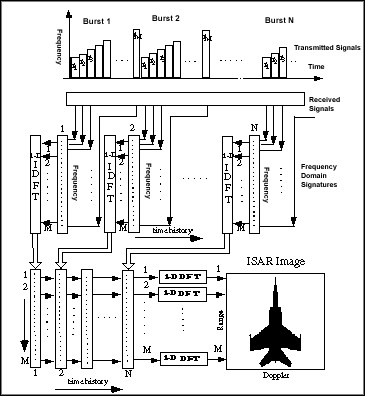
Figure 1. The Conventional Stepped-Frequency ISAR Imaging System

By using DFT to compute the Doppler frequency, it is necessary to assume that the Doppler frequency is constant over the imaging time duration, so the extraneous phase term is neglegible. However, the assumption of constant Doppler frequency is not true. The Doppler frequency varies in time because of the nonuniform motion of the target. The global Fourier spectrum, computed by DFT, often leads to a blurring image.

The mechanism of the cause of blurring image has been recognized for a long time. Over the years, many attempts, such as shorter observation time, subaperture method, and super-resolution, have been made to obtain the time-varying spectrum in the hope of enhancing image resolution. However, none of them can completely resolve the blurring problem. The fundamental requirement for the desired technique is that the prospective algorithm has to give a good estimation of the instantaneous frequency of the time history series. Moreover, it must possess a high resolution in the time and frequency domain simultaneously. While neither Fourier transform nor super-resolution meets those requirements, the recently popularized bilinear transformations are very promising alternatives. In this paper, we introduce a new ISAR system, in which the Doppler frequencies are computed by the joint time-frequency transform (JTFT).

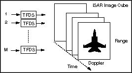
Figure 2. A Proposed JTFT Based ISAR Imaging System. Note, that the only difference between the new and traditional ISAR systems is that the Doppler frequencies in the proposed ISAR are computed by the joint time-frequency transform rather than by DFT.

Figure 2 illustrates the proposed ISAR imaging scheme. Because the Doppler spectrum is computed by the JTFT, one image frame in the traditional ISAR system is now decomposed into several instantaneous time frames. Our extensive testing on both simulated and real data indicates that the JTFT significantly improves the traditional ISAR performance. To demonstrate the effectiveness, Figure 3 compares the simulated image of a MIG-25 obtained by the traditional ISAR and one of the multiple frames generated by the new ISAR. While the DFT-based ISAR image is blurred due to the fast rotation of the aircraft, a clear aircraft image is observed from the JTFT-based ISAR. As far as the authors are aware, such results have not been achieved by any current methods mentioned earlier. Moreover, it is important that the only difference between the new ISAR and the traditional ISAR is that the JTFT replaces the DFT. The traditional ISAR can be easily up-dated without significantly altering the existent hardware structure. Because of the effectiveness and simplicity, we believe that the technique discussed in this paper will strongly impact future ISAR processor design.

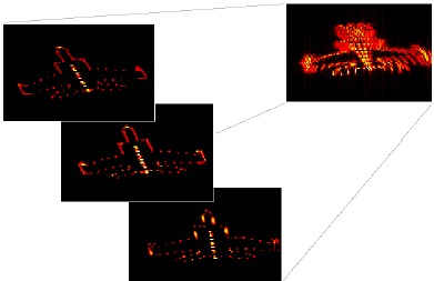
Figure 3. MIG-25 ISAR Images Computed by DFT (right) and JTFT (left). Time-frequency transform successfully resolves the blurring problem caused by the global spectrum.

It has long been recognized that time-varying signals (e.g., chirp-type signal) are more easily recognized in the joint time-frequency domain than in either the time or the frequency domain alone. This observation has inspired researchers to pursue detection algorithms based on signal joint time-frequency representations. Unfortunately, the mapping of a time domain signal into the joint time-frequency domain is computationally intensive, prohibiting real-time detection via the joint time-frequency representation for applications having bandwidths greater than audio.

In many real-time detection applications, the matched filter is employed, which is optimal in the sense of maximum signal-to-noise ratio (SNR), and amenable to analog hardware implementation with bandwidths in excess of 20 MHz. Unless the object signal is known precisely, however, the design of the time waveform template is impossible, especially when the desired signal is embedded in noise. This paper discusses a general methodology of deriving time templates for deterministic waveforms, usually with a number of parameters, using joint time-frequency representation. Once the waveform template is obtained, sparse-matched filter banks can be used to capture signals of interest. The effectiveness of the proposed technique is demonstrated by an example in radio physics—real-time detection of transionospheric signals.

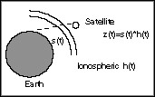
Figure 4. z(t) can be considered as the convolution of s(t) and h(t).

In radio physics, there is great interest in detection and estimation of impulsive signals which have been dispersed by transmission through ionized media. These impulsive events are an important aspect of research in climate change and global electrodynamics. As shown in Figure 4, some signals are collected by satellites currently. The received signal z(t) is traditionally modeled as the convolution of a quasi-impulsive s(t) (broadband over the VHF, S(f) » C, where C denotes a real-valued constant) and an ionospheric channel impulse response h(t) (which can be described as a nonlinear chirp function). Hence, the Fourier transform of the received signal is

In other words, z(t) is similar to the ionospheric channel impulse response h(t) and therefore is also a chirp-type signal. Figure 5 illustrates the preprocessing actually taking place in the DOE/Los Alamos Laboratory satellite Alexis.

Figure 5. The mixer reduces the required sampling frequency from 200 MHz to 150 MHz.

Normally, x(t) of interest persist for several microseconds, and long dead times exist between events. Without an accurate trigger, the great majority of data collected on a satellite will not contain any signals of interest. Since the signal bandwidth is as high as 75 MHz, it is impossible to store all the data in the satellite or send it back to the earth station. A critical issue required in an effective transionospheric radio sensor is first to detect the presence of x(t), and then to capture the time series representing it, thereby reducing the amount of data needed for transmission to earth. However, it is not trivial to accurately detect x(t), because in many situations the SNR of x(t) is less than 1. Although x(t) can be recognized in the joint time-frequency domain, for such high sampling rates the computations required for joint time-frequency transformation are above 10 GFLOPS, at the limit of super computer technology. The alternate technique described in this paper, using sparse-matched filter banks, provides a means of achieving the same result, with miniature, low-power electronics.

Without loss of generality, assume the time-varying signal of interest to be w(t) = A(t)exp{jj(t)}, where j(t) denotes the phase. The first derivative of phase j¢(t) is the so-called instantaneous frequency, which is time dependent. Now transform an ensemble of representative time functions x(t) into the joint time-frequency representation P(t,f). The desired signal, a chirp-type signal, is more easily recognized in the joint time-frequency domain because many continuous-wave or impulsive interference sources can be removed. Then the enhanced P(t,f) is projected into f(t) as shown in Figure 6, where f(t) is a multiple value scatter function in the time-frequency plane. If the mapping of x(t) to P(t,f) is done properly, then the curve f(t) should be a good approximation of signal instantaneous frequency. Finally, a conventional curve-fitting routine can be used to determine an analytic formula for j¢(t) from the scatter function f(t). For each member of the ensemble of representative time functions x(t), a variation of the fit parameters will be observed. Therefore a family of filter functions will be described, spanning the variation of a few parameters in the model function for j¢(t). Due to the nature of chirp convolution, significant correlations occur over large spans of the dispersion constant, K, allowing a sparse set of K values to adequately span the desired chirp function space.


Obviously, the particular joint time-frequency representation used will affect the accuracy of this procedure. To reliably estimate j¢(t), the joint time-frequency representation should have the following properties: (1) insensitivity to noise and artificial interference, so that the desired signal can be distinguished above background; (2) the observed trajectory of the signal in the time-frequency plane should be numerically close to the instantaneous frequency j¢(t). The spectrogram is indeed less sensitive to noise and interference, but the corresponding estimation j¢(t) is subject to the selection of the windows. As an alternative, the time-frequency distribution series (TFDS), also known as the Gabor spectrogram in industry, which is derivative of the Wigner-Ville Distribution, is proposed here. Since the performance of the TFDS is less sensitive to the selection of parameters (for example, the Gabor basis function), it is particularly useful when less information about the signal of interest is available.

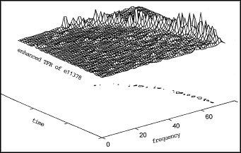
Figure 6. Instantaneous Frequency Estimation

Based on the ensemble of time functions x(t) collected, the best model for the instantaneous frequency function is found as:

where is equal to the mixer frequency is the curvature parameter of the model. flc = 100 MHz. The parameterK is the curvature parameter of the model.

For simplicity, and without any consistent amplitude variation observed, we further define the magnitude A(t) as a rectangular window. By simple mathematical manipulations, finally we obtain the time template:

where U(t) denotes the unit step function. It should be noted that wK (t)is closely related to the ionospheric channelimpulse response h(t) obtained in physics. This lends credibility to the technique presented in this paper as a means of finding the correct dispersion function from the joint time-frequency representation.

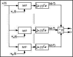
Figure 7. Block Diagram of RF detector

In Figure 7, one potential implementation of a detector is shown in block diagram form. To process the outputs of the matched filters, which are extended oscillatory functions, a rectifier and filter, or energy detector, is added, in which the integration time period sets to 1 ms (150 samples). The detector outputs “1” when any of the matched filters exceeds a detection threshold, to be determined by the observed noise levels. Our numerical simulations show that all signals collected in a day of ionospheric variation can be reliably detected by no more than
16 templates WK(t), where K = 0, 5, 10... 75 MHz. This new method of detection significantly improves false alarm rates of conventional undispersed filter banks now used in ionospheric work. As further refinement of the algorithm takes place, a hardware implementation is in conceptual design, as a bank of FIR surface acoustic wave or digital CMOS structures. We believe the techniques described in this paper will be important in many physical measurements, wherever a parametric model of low order can be used to describe a variable signal with uncertain arrival time.

Economic data is traditionally considered an erratic and noisy time series. The orthodox economic theory asserts that economic movements are random walks and basically no regularity exists. Therefore, the predominant analysis tools used in the economic community have been statistical analysis, such as the auto regressive model (AR). Instead of trying to explore the regularities, economists traditionally use the empirical data to fit the artificial linear models. For a good fit, the real data has to be “prewhitened” (in other words, we need to make the data even more noisy). However, the stochastic models in general are only capable of calculating “mean” and “variance,” which are not adequate for most business applications.

On the other hand, experience from our daily life tells us that there are certain business cycles, though their length may change in time. For example, most economists believe that since World War II, the business cycle in the U.S. has been about four to seven years. Unfortunately, neither stochastic analysis nor traditional Fourier analysis support their hypothesis. Therefore, we are motivated to seek new methods to better understand the economic movements.

Recently, we applied the joint time-frequency analysis (JTFA) techniques, developed by National Instruments, with encouraging results. Unlike the traditional Fourier analysis, the joint time-frequency analysis methods characterize the time series in the time and frequency domains simultaneously. Applying JTFA, we know not only what kind of cycles exist, but also when they occur and how long they last. While the meaningful cycle (the cycles that last for a certain period of time) is concentrated in the joint time-frequency domain, the random noise tends to evenly spread into the entire time-frequency plane. Consequently, the JTFA possesses higher signal-to-noise ratio.

As our extensive tests indicate, for the majority of economic data there are certain regularities. They could be very obvious if a proper pre-processing is applied. Here, we propose an entirely new method to analyze economic data:

1. Instead of prewhitening, find a smooth trend curve to fit empirical data so that the residual contains as many meaningful cycles as possible;

2. While the smooth curve presents long term trends, the residual can be used to analyze short term behavior Figure 8 depicts the analysis results of the S&P 500 Stock Price Index. The bottom plot represents the time series (jagged line) and the trend (smooth line). The right-hand plot depicts the power spectrum of the residual, the difference between the time series and the trend. Although the spectrum indicates which frequency components the residual contains, it does not tell when they occur or how long they last. Because only those frequencies that last a certain period of time can be considered a meaningful cycle, there is no way to determine the business cycle from the spectrum alone.

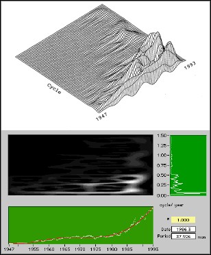
Figure 8. S&P 500 Stock Price Index Analysis

The middle (intensity) and upper (three dimensional) plots show the results of using JTFA on the signal residual. The horizontal and vertical axes correspond to the time and the period of the business cycle, respectively. This particular JTFA method uses the Gabor spectrogram (also known as the time-frequency distribution series) developed by National Instruments. Compared to the other JTFA techniques, the Gabor spectrogram obviously has better resolution and less cross interference. It therefore seems most suitable for our applications.

Figure 9 depicts the results of the analysis of the U.S. unemployment rate. Again the lower and right-hand plots represent the time series and the power spectrum of the residual, respectively. The middle and upper plots are the results of the JTFA techniques.

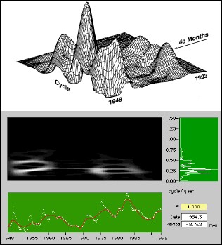
Figure 9. Unemployment Rate Analysis

As illustrated in Figures 8 and 9, both sets of economic data have very clear patterns. In the S&P 500 illustration, there is a long cycle (about 256 months, over the past 50 years), a medium cycle (about 38 months), as well as a short cycle (about 25 months). The long cycle reflects the slow pace of structural changes. The medium cycle is crucial for strategically economic decision. The short-term cycle is critical for speculative investors. The most interesting observation is that the dominant cycle for the unemployment rate is 48 months, the exact length of one term of the U.S. president. This coincidence probably means that the U.S. economy is closely related to political changes.

At present, only preliminary research has been conducted, but the potential for using JTFA for economic data analysis is obvious. This trend may lead to a revolution in the economic community.

The ultrasonic method is one of the most powerful methods to nondestructively examine the hidden defects of materials. Ultrasonic signals are typically nonstationary in nature because of the lack of uniformity in the generally complex material properties. It has been recognized for a long time that the use of time domain or frequency domain information alone is often inadequate to characterize the defects. In searching for time-frequency analysis methods, we found the Gabor spectrogram, developed by S. Qian and D. Chen at National Instruments, to be the most suitable in providing the desired joint time-frequency domain information.

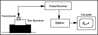
Figure 10. A Typical Ultrasonic Inspection System

The following example illustrates the detection and classification of hidden geometrical defects in aluminum blocks. The test system, shown in Figure 10, consists of a pulse generator (or pulsar), a pulse receiver, a transmitting transducer, a receiving transducer, and a digital oscilloscope. The pulse generator and receiver are usually sold together as a single unit with a built-in amplifier. In addition, most commercially available ultrasonic transducers can be used both as transmitters and receivers of ultrasonic waves. The pulse generator sends out an electrical pulse that is converted into a mechanical pulse in the transmitting transducer (the range of frequency of this pulse extends from about 0.2 to 50 MHz). The pulse thus generated is then coupled into the test specimen. An echo reflected from any acoustic mismatch in the material is converted into an electrical pulse received by the pulse receiver. The echoes received are then amplified and displayed on the oscilloscope. In this example, the center frequency of the transducer is 15 MHz. The sampling frequency is set to 100 MHz.

The test samples are T15A0, without any defects, and T15A1, with a flat top defect. Usually, it is rather difficult to distinguish the flat top defect from the normal material. Figures 11 and 12 depict the echo signals corresponding to two different test samples. The bottom plots are the time waveforms of the echo signals. The right plots are the corresponding spectra. You can see that the features obtained from time waveforms or spectra alone do not clearly distinguish between the good sample and the defective sample. The middle and upper plots are intensity and three-dimensional representations of the 3rd-order Gabor spectrogram, the joint time-frequency analysis algorithm from National Instruments. They clearly distinguish between the two samples. The upper plots are centered around the 15 MHz transducer frequency. Note that the echo of T15A0, centered at about 12.5 MHz, has a narrower bandwidth and longer time duration than the equivalent echo from T15A1. The narrower bandwidth may explain the fact that the structure of the defect-free material is relative uniform. The longer time duration may indicate the system resonant is close to the center transducer frequency and thereby the damping factor is small. Although, the total energy in the vicinity of 15 MHz is almost the same in the two plots, the energy distribution patterns in that area are clearly different . This observation is undoubtedly useful for defect classifications.

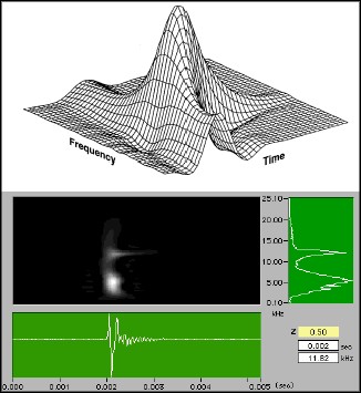
Figure 11. Analysis Results from Defect-Free Sample (T15A0)

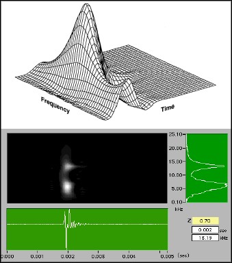
Figure 12. Analysis Results from Defective Sample (T15A1)